
 Version 3.0
Ground source heat pump simulation and ground loop sizing
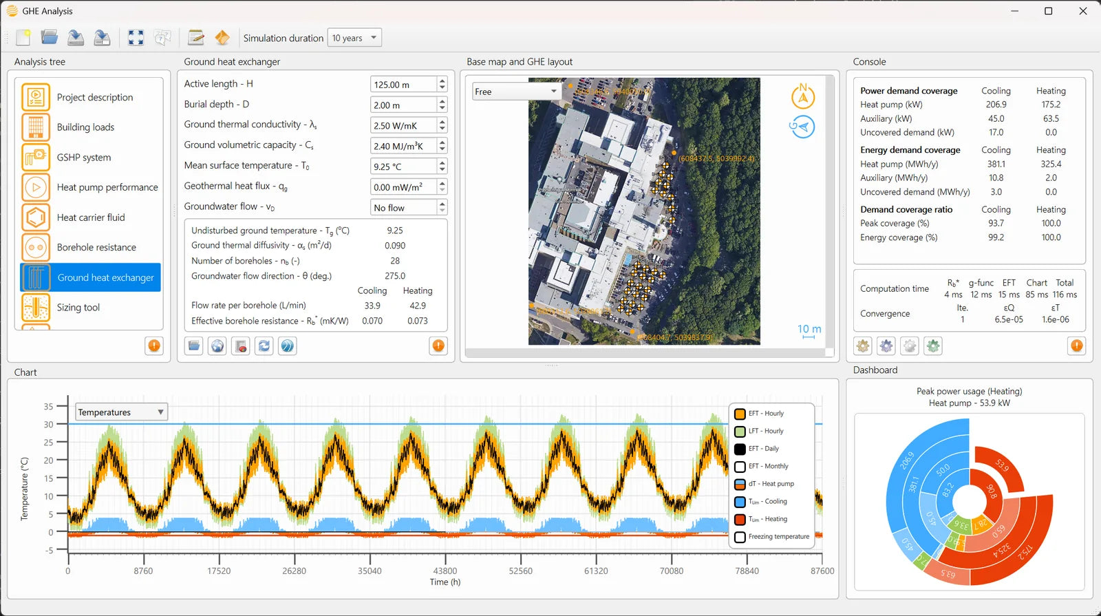
GHE Analysis is ground source heat pump simulation software: it sizes the ground loop and simulates the entering fluid temperature hour by hour, over a design horizon of one to fifty years and up to 625 boreholes. Drag a borehole across the site map and the g-function of the field is recomputed before you let go.
Windows 10 or later and macOS 14 or later. Nothing runs in the cloud.
You design by moving boreholes, not by editing a parameter file.
A borehole field is not specified, it is arranged. Import the site map, georeference it on four points, and place the boreholes where the parking, the foundations and the future building actually leave room. Select a group with the mouse and move it, rotate it, stretch it. Double-click to add one, Backspace to remove a selection.
Every one of those gestures recomputes the g-function of the field, automatically and in a fraction of a second, while the mouse is still down. Not a lookup, and not the nearest entry in a catalogue of predefined configurations: the response of the field as you have just drawn it, irregular spacing and all.
You are not preparing a case to run later. You are reading the thermal consequence of a layout decision at the moment you make it.
Groundwater flow, inside the g-function
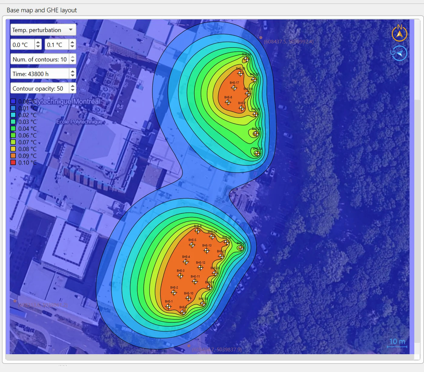
Most design tools treat the ground as still. GHE Analysis carries groundwater flow through the whole simulation instead, set by direction and Darcy flux. Turn the flow direction with the wheel, in five-degree steps, and watch which boreholes fall downstream.
One tool, every GSHP configuration.
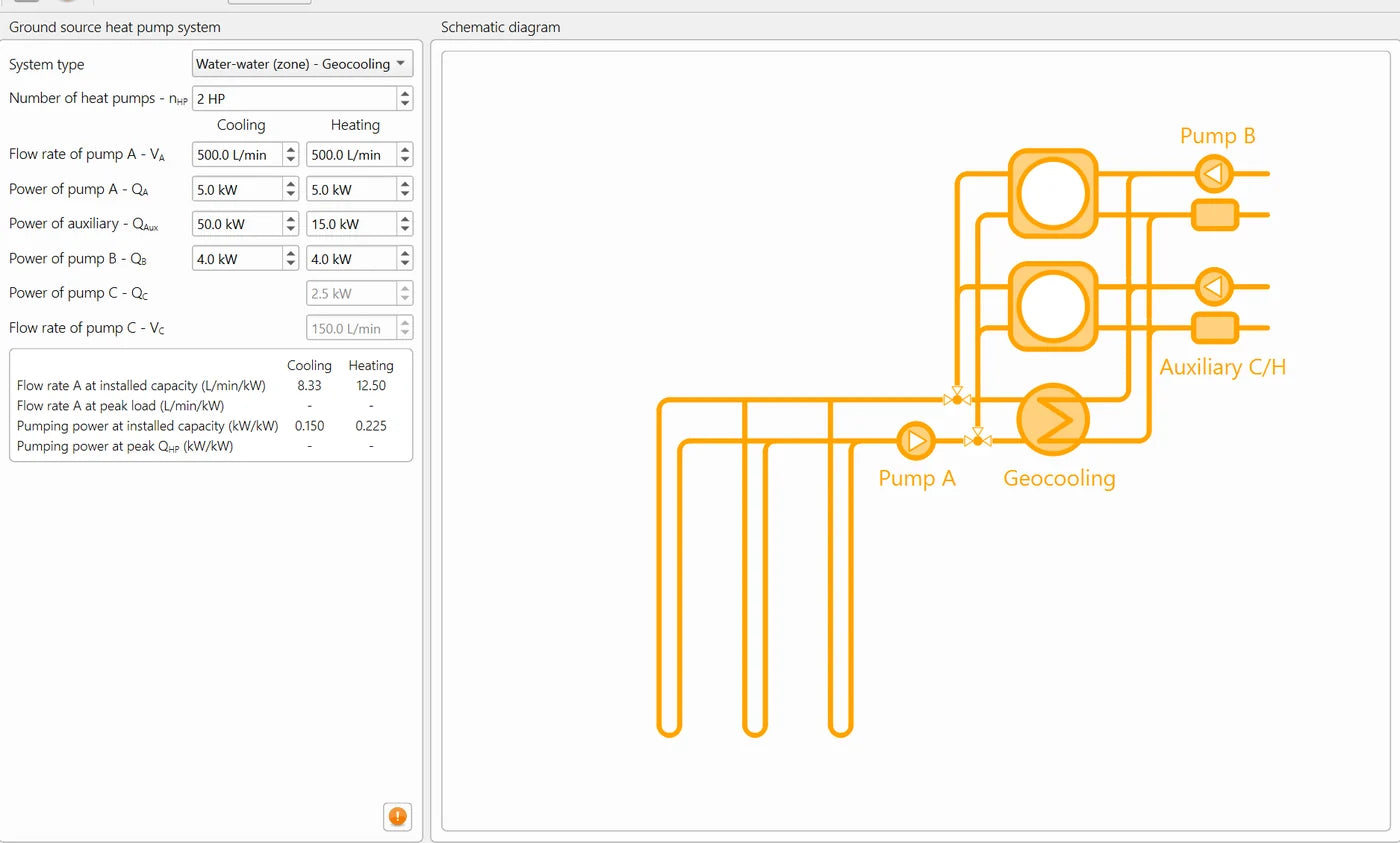
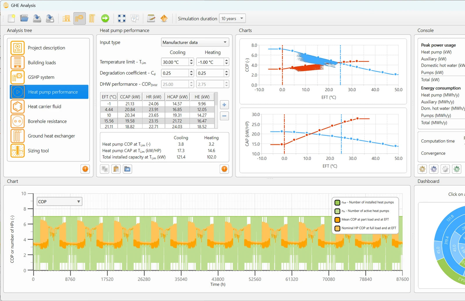
GHE Analysis models the ground loop as one part of the mechanical system, not as an input you guess and hope holds. Water-to-air zone units, water-to-water zone units, and a central water-to-water plant with integer staging are carried as three distinct archetypes, each with its own dispatch — which units run, at what part load, and what an oversized or undersized field does to entering fluid temperature and COP over the life of the plant.
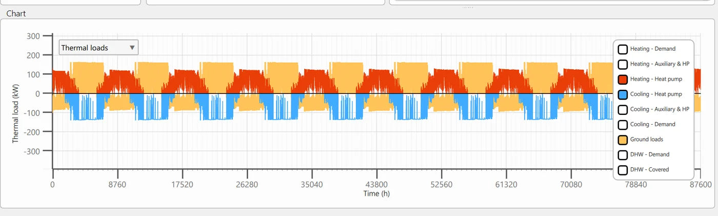
Geocooling, also called free or passive cooling, takes the building heat straight to the ground with the compressors off — often the single largest efficiency gain available in a cooling-dominant building. Domestic hot water is covered only as far as the heat actually available allows, never assumed, and heat pump COP and capacity follow the temperature they actually see, with a part-load degradation coefficient a straight-line COP curve would miss.
Hybrid systems are simulated the same way, hour by hour. Cap the field at the smaller of the heating and cooling loads, and let a fluid cooler or an auxiliary heater carry the peak of the other: GHE Analysis dispatches that auxiliary equipment alongside the heat pumps rather than applying a rule-of-thumb sizing margin, so you see exactly how much field the hybrid strategy buys back, and shift capital from permanent drilling to equipment you can inspect, service and replace.
Specifications
The lines below are the ones that decide a design. Each is a panel of the application, and each has its own chapter in the manual. See the full feature table.

Layout and geometry
- Import a site map, georeference it on four points, and place boreholes directly on it
- Move, rotate and stretch a group of boreholes; azimuth and dip set per borehole
- 3D borehole viewer and 2D thermal plume viewer, with a temperature probe at any point

Ground heat exchanger models
- Single and double U-loop, adjacent and diagonal inlet
- Coaxial borehole heat exchanger
- Inclined boreholes, and standing column well with bleed control

Loads, equipment and system
- Building or ground thermal loads, hourly and monthly
- Temperature-dependent COP and capacity, with part-load degradation
- Geocooling and domestic hot water, across three system archetypes

Simulation and sizing
- Hourly entering fluid temperature over the full design horizon
- Regional groundwater flow, by direction and Darcy flux
- Borehole resistance re-evaluated at every operating point, for temperature and flow rate

Energy and cost
- Operating-energy cost with a flexible tariff engine, and capital cost of the project
- Circulating pump and auxiliary loads carried in the energy balance, not left out of it
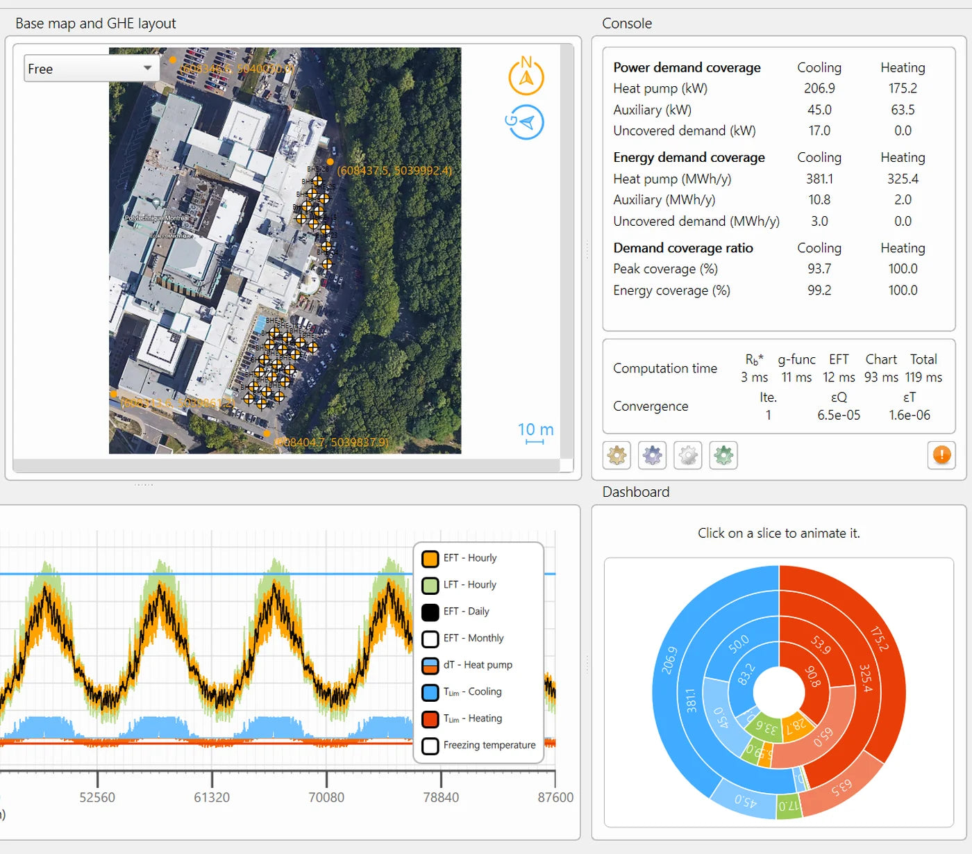
- Annual energy balance as a Sankey diagram

Results and export
- Seven chart views, from fluid temperature to the g-function
- Automatic CSV export on save, hourly simulation results included
- Self-contained .ghe project file, and context help on every panel
Sizing that tells you why
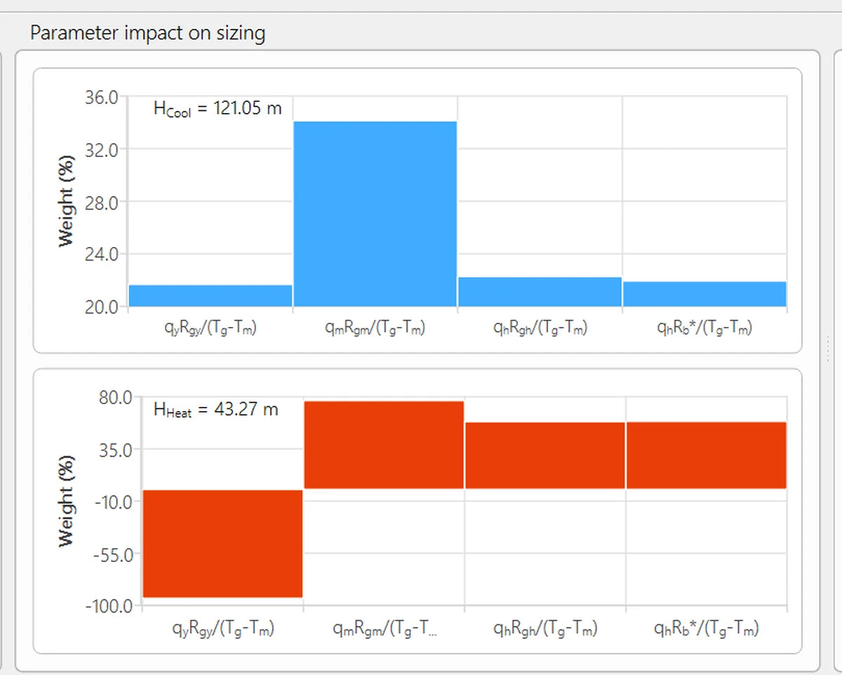
The sizing tool applies the ASHRAE alternative method and breaks the required length into four contributions: the annual pulse, the monthly pulse of the peak month, the hourly peak, and the borehole resistance.
Read together, the four columns say why a field is the size it is. A tall first column means an unbalanced load, and no amount of extra drilling fixes that. A tall last column means the borehole resistance is worth improving before adding a single metre.
Size here, carry the longer of the heating and cooling lengths into the field layout, then confirm with the full simulation.
Reading the result
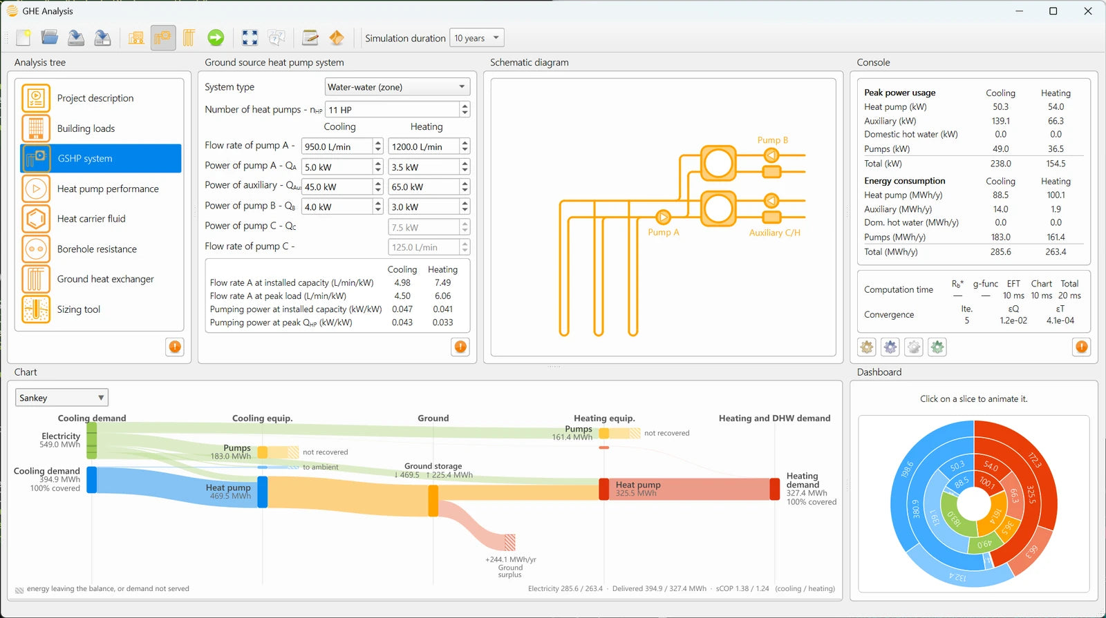
- The Sankey diagram, new in 3.0, condenses a year of operation into one picture: where the energy comes from, and where it ends. Two bars carry most of the story, demand the equipment could not meet, and the annual surplus or deficit left in the ground.
- Thermal plume contours at any simulation time, with a temperature readout wherever you click.
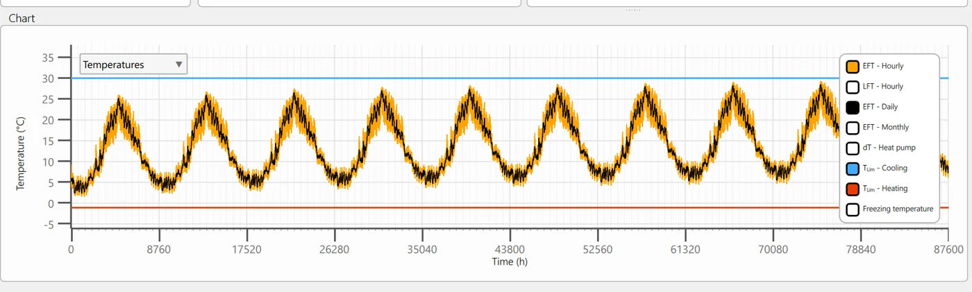
- Entering fluid temperature, hourly, daily and monthly on one axis, with the heating and cooling limits drawn in. A profile that drifts year after year is a field going out of balance, visible long before it becomes a complaint.
- The g-function, on a logarithmic time axis, its long-time plateau is the single number that says the most about a layout.
- Effective borehole resistance against time, where the shift from laminar to turbulent flow shows up as a visible spike.
Seven chart views in all, and none of them is a dead end: saving the project writes the hourly results out as a CSV beside it, automatically, so the run you just read can be taken into a spreadsheet, a report or a script without being repeated. Every chart, in the manual.
One application, one download
 TRT Analysis
 GHE Analysis
 GLN Analysis
GHE Analysis is one module of Analysis Suite. TRT Analysis interprets the thermal response test, GHE Analysis designs the ground loop, and GLN Analysis balances the network that connects it. They share the heat-carrier fluid, the project record and the console.
A parameter measured in one module can be carried into the next, and you choose which technique's value travels. A ground conductivity fitted from a response test does not have to be retyped to be used.
Licensing
GHE Analysis is in every Analysis Suite licence, from the smallest tier up. What changes between tiers is the size of the field you may design, never the method behind it: a residential loop of a few boreholes is modelled by the same kernel, and to the same standard, as a six-hundred-borehole institutional field.
Free for academic research and classroom use — see the academic licence.
Questions
What does GHE Analysis compute?▾
GHE Analysis sizes the ground loop and simulates the entering fluid temperature hour by hour, over a design horizon of one to fifty years and up to 625 boreholes. The g-function of the field you draw is recomputed automatically, rather than looked up from a catalogue of predefined layouts.
Can I move boreholes on the layout and see the result update live?▾
Yes. Moving a group of boreholes recomputes the field's g-function, the fluid temperature simulation and every chart — together, before you let go, not as a staged sequence you wait through.
Does GHE Analysis account for groundwater flow?▾
Yes, and throughout the entire simulation, not as an add-on: regional flow, set by direction and Darcy flux, acts on every borehole for the full design horizon. Among geothermal design tools, this native integration is unique to GHE Analysis.
Can it model hybrid or peak-shaving systems?▾
Yes — water-to-air, water-to-water and hybrid systems are all simulated hour by hour, with geocooling and domestic hot water integrated rather than left as manual adjustments, and heat pump COP and capacity interpolated from the entering fluid temperature the loop actually delivers, not read off a nameplate curve. A fluid cooler or auxiliary heater is dispatched alongside the heat pumps rather than sized by a rule-of-thumb margin, so you see exactly how much field the hybrid strategy buys back.
Is GHE Analysis hard to learn?▾
No. The interface is built for a fast, guided first session, not a course of video tutorials before you can start a design. Context-sensitive help is one click away on every panel, and the full manual is available online or as a PDF whenever you need more depth.
How many boreholes can it model?▾
GHE Analysis integrates up to 625 boreholes directly, at depths up to 500 m, in regular or fully irregular layouts — larger fields, up to 3,000 boreholes, are available on request. The g-function is computed for the field as drawn, never looked up from a catalogue of predefined configurations.
Have GHE Analysis's results been validated?▾
Yes. The application ships with 137 verification scenarios covering every stage of the calculation — borehole resistance, g-functions, sizing and fluid temperature — each checked against independent published methods and reference tools. Every scenario runs from the Examples and verification menu, so the comparison isn't just a claim.
Read further
- How to design an energy-efficient ground source heat pump systemThe decisions that actually move the efficiency, in the order they are made. →
- From sizing to simulationWhy a sized length is where the work starts, not where it ends. →
- Reducing borehole thermal resistanceWhat changes the resistance, and what only looks like it does. →
- The GHE Analysis manual, in full14,000 words and 20 figures, every method traced to its source. →