
 Version 3.0
Hydraulic design of ground loop networks
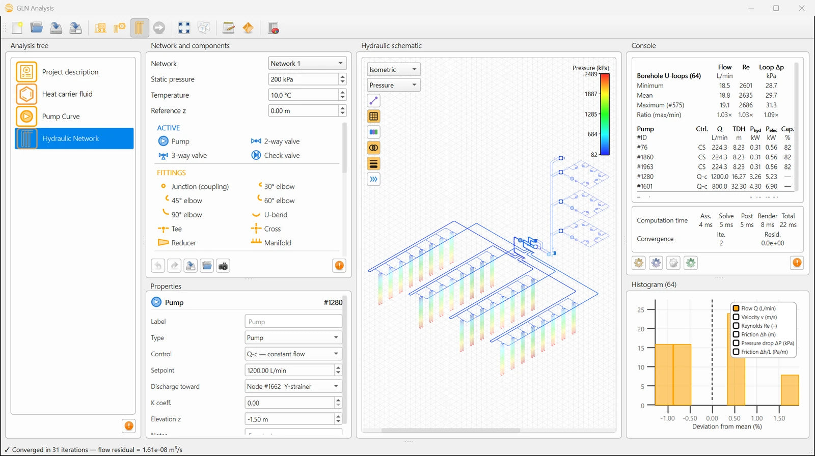
A borehole field can be sized correctly and still give a disappointing seasonal performance if the piping network around it is poorly designed. GLN Analysis solves that network as a diagram — flow, friction, pump head, and the balance between borehole loops — and keeps it solved as the design changes interactively.
Windows 10, Windows 11 and macOS. Nothing runs in the cloud.
Why it exists
A great many ground source heat pump systems never deliver the savings they were sold on, and the reason is often not in the ground but in the pump. A circulator two sizes too large, or a network laid out so awkwardly that only a large circulator can push the design flow through it, converts electricity into heat and friction for the whole life of the installation, and that parasitic power is subtracted directly from the benefit the system exists to produce.
Flow, animated on the drawing
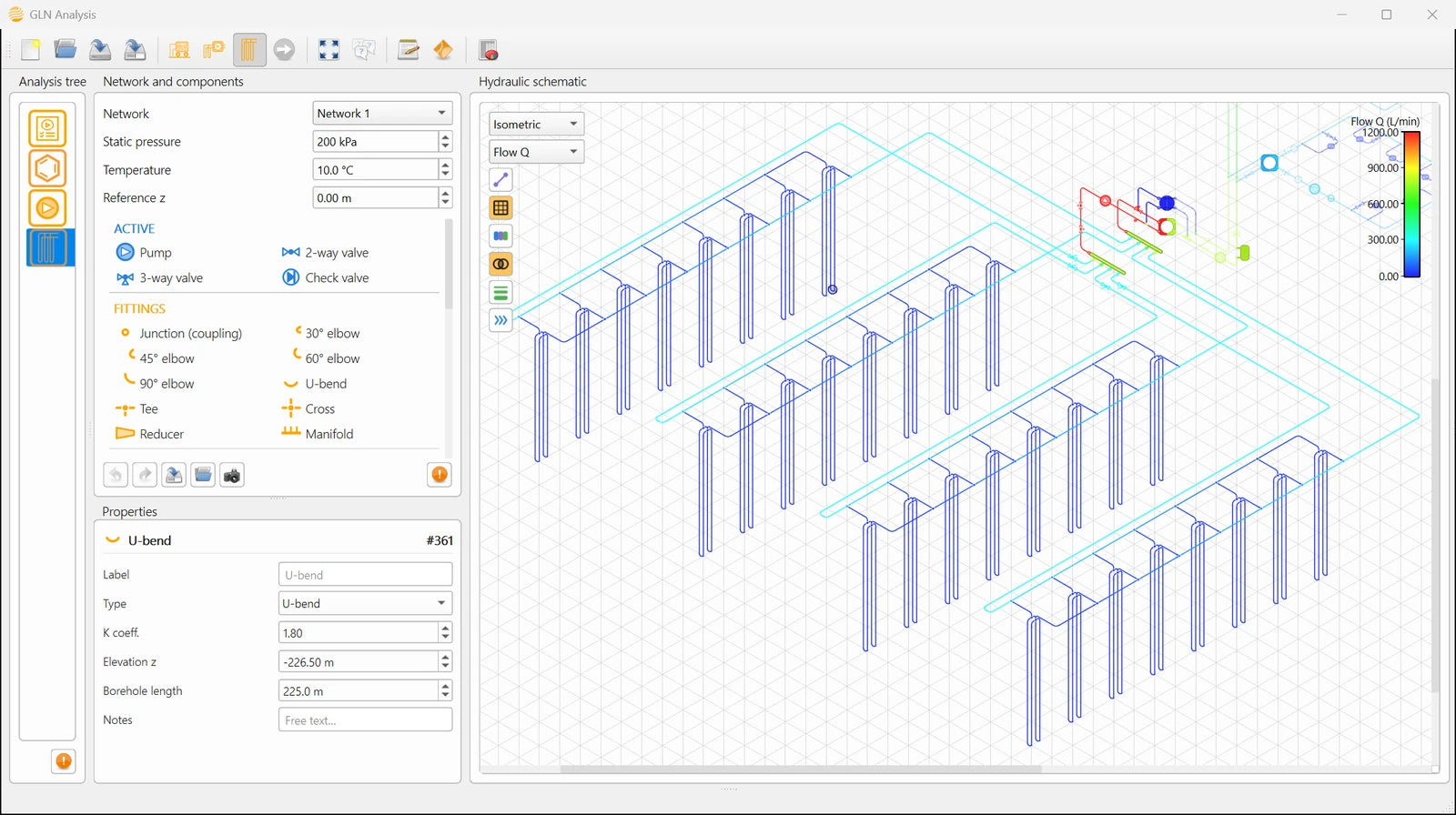
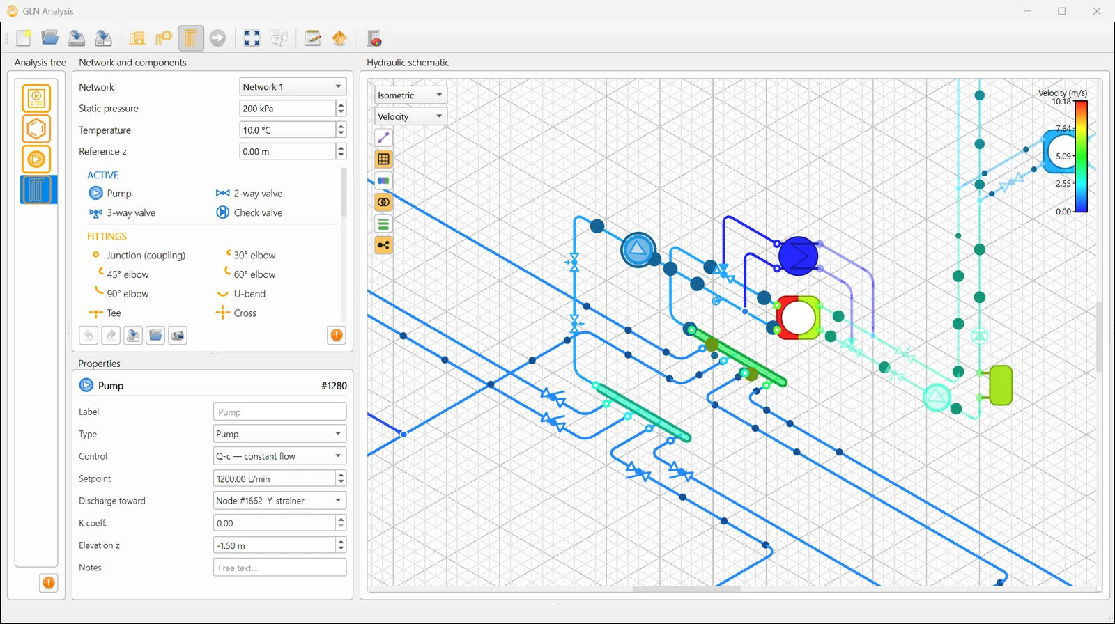
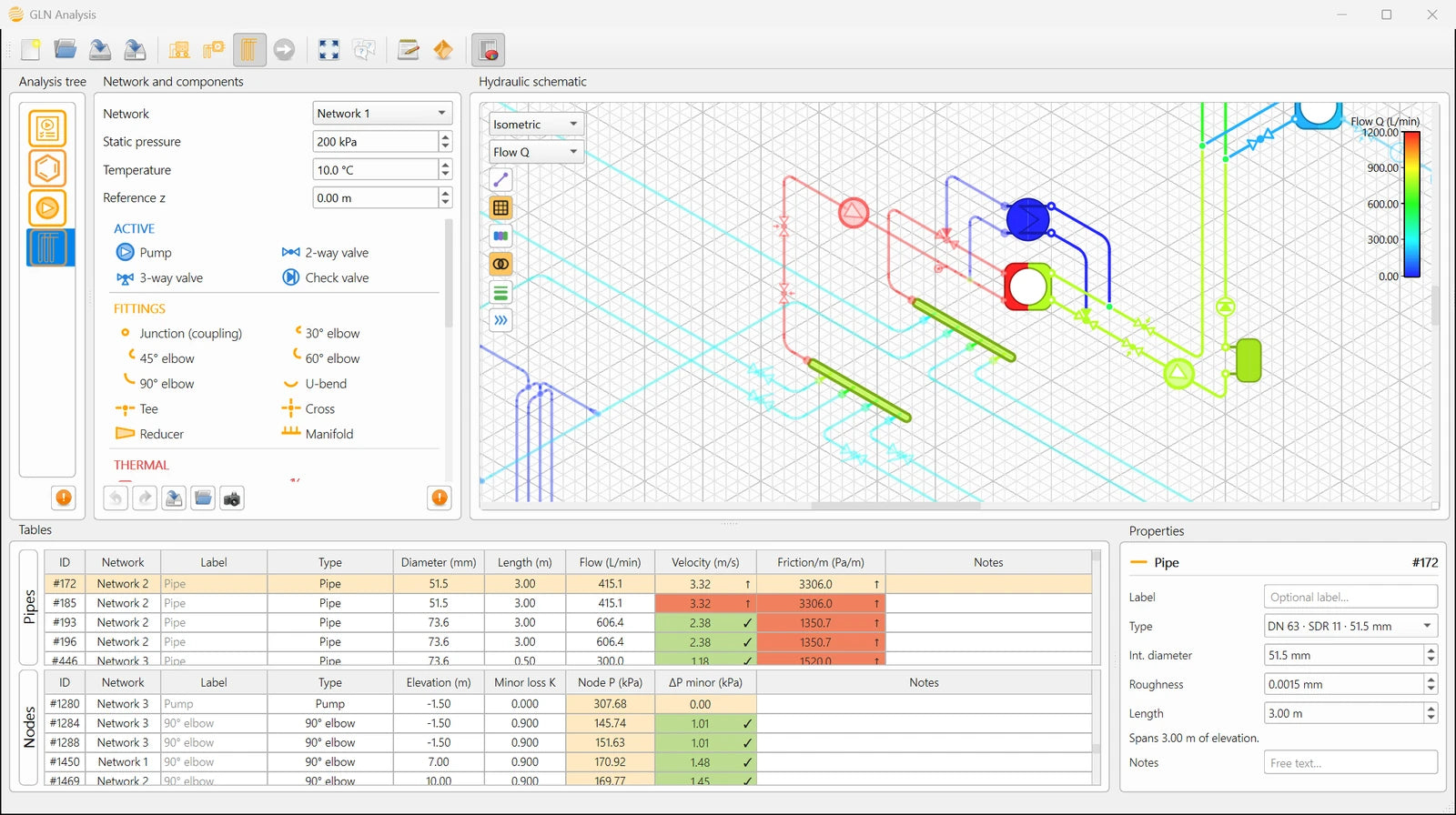
Once a network is solved, GLN Analysis can animate the result on the canvas itself: beads travel along each pipe, their size carrying the flow rate and splitting at every branch the way the fluid does. A second mode traces the same solution as marching dashes, sized by velocity instead.
What it computes

Drawing the network
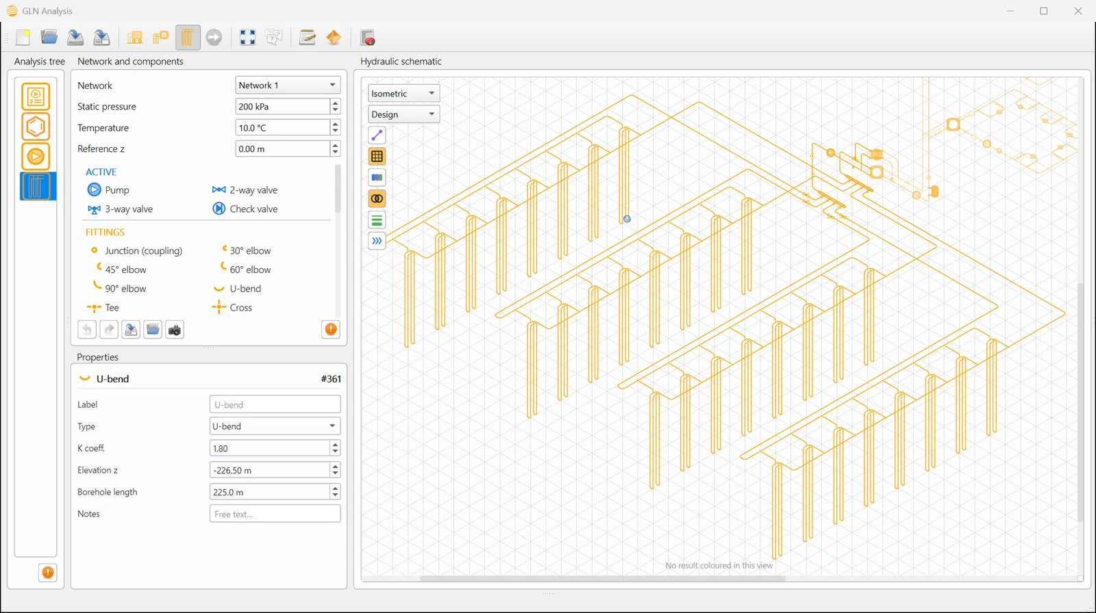
- The network is drawn as a piping and instrumentation diagram: a node for every component, an edge for every pipe
- 35 component types across seven families — active, fittings, thermal, ground heat exchanger, instrumentation, storage & safety, treatment — each in its own colour on the palette
- Any selection saves as a reusable archetype, so a plant room or a borehole head drawn once can be dropped into any later project
Solving it
- Newton-Raphson solution of the mass balance at every free node
- Darcy-Weisbach distributed losses with a Swamee-Jain friction factor, valid from laminar to fully rough turbulent flow
- Minor losses as K·ρv²/2, seeded by component type from published values
- Several independent networks in one drawing, each with its own pressurization point, fluid and temperature

Pumps and fluids
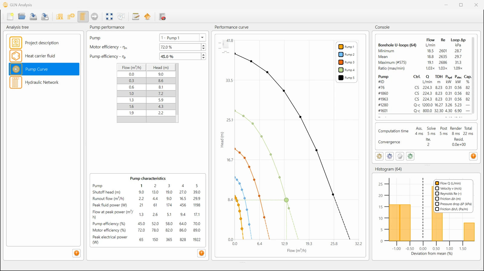
- A pump library described by manufacturer H-Q points, completed to shutoff head and runout flow, with separate hydraulic and motor efficiencies
- The solver finds where each curve meets the resistance of its circuit, and reports flow, head, fluid power and electrical draw at that point
- Variable-speed control at constant speed on the curve, at constant head, or at imposed flow
- Water or one of four antifreeze solutions through the Melinder correlations, at each network's own temperature
Checking the design
- Velocity and friction gradient flagged against the recommended windows, 0.3 to 2.5 m/s and 100 to 400 Pa/m, per pipe and rolled up in the console
- Balancing indicator: borehole U-loops are detected geometrically, and the ratio of the highest to the lowest loop flow is reported as the balancing figure of the field
- Reynolds number per element, which says whether the exchange in the borehole is the turbulent flow the thermal design assumed
- Pressure, velocity, head or elevation mapped onto the drawing itself

Catalogues and export
- 35 component types across seven families, each seeded with a default loss coefficient checked against Crane, Idelchik, ASHRAE, PPI and GF published tables
- 49 pipe catalogue entries, metric (ISO 4427) and imperial (ASTM D3035/F714) series, with bore and roughness set from the same standards rather than typed by hand
- Automatic CSV export of the full per-pipe result table on every save — flow, velocity, Reynolds number, friction factor and pump operating points — with no separate export step
Every entry in the drawing palette — the same seven families, the same order.
 Pump
 2-way valve
 3-way valve
 Check valve
 Junction
 30° elbow
 45° elbow
 60° elbow
 90° elbow
 U-bend
 Tee
 Cross
 Reducer
 Manifold
 Heat pump
 Auxiliary heat/cool
 Heat exchanger
 Radiator
 Fan-coil unit
 Single-U borehole
 Double-U borehole
 Coaxial borehole
 Flow meter
 Temperature
 Pressure
 Energy meter
 Expansion vessel
 Reservoir
 Buffer tank
 Fill / make-up valve
 Y-strainer
 Air separator
 Dirt separator
Reading the checks
Each check sits in the cell of the number it judges — the colour is the verdict, not a separate report to read. A pipe outside its velocity or friction window, a loop taking more or less than its share of flow, or a section that will not purge clean: all three are visible on the same drawing you are already looking at, and they update the moment the design changes.
What makes it different
A ground loop is judged on four questions, and this answers them on the actual drawing.
Does every borehole get its share of the flow? Is that flow turbulent at the heating peak? Is each pipe the right size? And what head must the circulating pump actually supply? The last one carries the operating cost of the installation for as long as it runs.
GLN Analysis answers those on the drawing rather than on a spreadsheet abstraction of it, and it keeps answering them as the design changes. The solution is a full nodal pressure field: the flow in every pipe, the velocity and friction gradient that decide whether a diameter is right, the Reynolds number, the head each pump must supply, and the spread of flow between borehole loops that says whether the field is balanced.
Three questions easier to answer before a system is built
Whether the pump is the right size, instead of one sized only to be safely large enough. Whether the antifreeze concentration chosen for thermal protection has moved the pump's operating point somewhere the circulator cannot follow — a hydraulic question a purely thermal analysis of the fluid never raises. And whether the network can be purged: GLN inverts the solve to find the total flow a purge pump must supply so the worst-served pipe in the field still reaches a target velocity, then names that pipe directly.
Interactive at the size where balance matters
The Jacobian is sparse and its pattern is analysed once. A five-hundred-borehole field, about two thousand unknowns, solves in a few tens of milliseconds. Hydraulic balance is a problem that shows up mainly in large fields, so the solver has to stay usable at that size to be useful at all.
Published methods
GLN Analysis's methods are not private correlations. Distributed losses follow Darcy-Weisbach, closed by the Swamee-Jain friction factor; minor losses are seeded from published handbook and manufacturer values; and the antifreeze correlations come from the standard thermophysical reference for secondary working fluids. Where field data exists, the solver is checked against it directly.
- ASHRAE, 2021. ASHRAE Handbook — Fundamentals, Ch. 22 "Pipe Design"; ASHRAE, 2023. ASHRAE Handbook — HVAC Applications, Ch. 35 "Ground-Source Heat Pumps and Geothermal Energy". American Society of Heating, Refrigerating and Air-Conditioning Engineers, Atlanta, GA.
- Crane Co., 2013. Flow of Fluids Through Valves, Fittings and Pipe, Technical Paper No. 410. Crane Co., Stamford, CT.
- Melinder, Å., 2010. Properties of Secondary Working Fluids for Indirect Systems, 2nd ed. International Institute of Refrigeration (IIR), Paris.
- Naicker, S.S., Rees, S.J., 2018. Performance analysis of a large geothermal heating and cooling system. Renewable Energy 122, 429–442.
One application, one download
 TRT Analysis
 GHE Analysis
 GLN Analysis
 is one module of Analysis Suite. TRT Analysis interprets the thermal response test, GHE Analysis designs the ground loop, and GLN Analysis balances the network that connects it. They share the heat-carrier fluid, the project record and the console.
The borehole field sized in GHE Analysis carries its geometry straight into the network drawing, so the field you just laid out does not have to be redrawn to balance it.
Licensing
GLN Analysis is included in every Analysis Suite licence, from the smallest tier up. The tiers set only the size of the network you may design. The calculation kernel is the same in all of them: a residential loop of a few segments is solved by the same nodal formulation, and to the same standard, as a five-hundred-borehole field.
Free for academic research and classroom use — see the academic licence.
Questions
What does GLN Analysis solve?▾
GLN Analysis solves the full hydraulic system, not just the ground loop: the mechanical room and the building's own distribution network are drawn and solved the same way — flow, velocity, friction and pump head in every pipe, plus the spread of flow between borehole loops that says whether the field is balanced.
Does it solve instantly from the drawing, or do I have to run a separate calculation step?▾
Instantly. Draw the system as a piping and instrumentation diagram — several independent networks in one drawing, if the project needs it — and the solution comes back before you've moved on: flow, velocity, friction and pump head in every pipe and network, even on a five-hundred-borehole field.
Has the solver been verified against an independent tool?▾
Yes. Its results are compared with EPANET, an independent solver, across dozens of reference networks — not tuned to agree with itself, but tested against a solver with no reason to.
Does it catch problems a purely thermal design would miss?▾
Yes — for example, whether the antifreeze concentration chosen for thermal protection has moved the pump's operating point somewhere the circulator cannot follow, a question a purely thermal analysis never raises.
Can it tell me whether a network will purge clean?▾
Yes. Instead of asking what flow a pump setting produces, the purge-velocity check asks the reverse: what total flow must be imposed so the worst-served pipe still reaches a target velocity, 0.61 m/s by default. GLN finds that flow by inverting the solve, names the limiting pipe, and can highlight every pipe on the drawing that meets or misses the target.
Is GLN Analysis hard to learn?▾
No. The analysis tree on the left takes you through a project in order, one panel at a time. Every panel opens its own help page, and each manual starts with a quick-start chapter that walks through a complete analysis. The manuals can be read in the application, online or as a PDF.

